Robot Learning - Sequence Modeling and Transformers

These are my notes from the Sequence Modeling & Transformers lecture of Robot Learning: From Fundamentals to Foundation Models (ETH Zürich, 263-5911-00L, Spring 2026, taught by Oier Mees). The lecture builds one long argument: a robot policy that looks at a single snapshot is not enough, so control has to become a sequence modeling problem; the Transformer is the tool we use for sequence modeling today; and once we have a Transformer that eats text and images, the remaining question is how to make it emit robot actions. The last part, action tokenization, turns out to be where the interesting failure modes live.

The slides below are from the lecture. Wherever a slide is drawn from a paper, the paper is linked right under it.

Why Reactive Policies Are Not Enough#

A reactive policy maps the current observation directly to an action, $\pi(a_t \mid o_t)$ . It is the simplest thing you can train, and it has three structural limitations:

One snapshot cannot capture the full state. A single camera frame does not tell you the velocity of a moving object, whether the gripper is already holding something, or what happened a second ago.
No memory. Anything that requires remembering an earlier event (which drawer was already opened, which half of a task is done) is invisible to the policy.
No action smoothness. Each action is chosen independently of the previous one, so consecutive commands can jitter.

The root cause is that robots almost never operate in a fully observed MDP. They operate in a POMDP (partially observable Markov decision process): the observation $o_t$ is only a noisy, incomplete view of the underlying state $s_t$ . Under a reactive policy the trajectory distribution factorizes as

p_\pi(\tau) = \rho(s_0) \prod_{t=0}^{T-1} \pi(a_t \mid o_t) \, P(o_{t+1} \mid o_t, a_t)

where every action depends on nothing but the current observation. To act well in a POMDP the policy needs to reason over history, that is, $\pi(a_t \mid o_{\le t}, a_{< t})$ . That is precisely an autoregressive model: predict the next element of a sequence conditioned on everything that came before. This is why the rest of the lecture is about sequence modeling.

From RNNs to Transformers#

The first generation of sequence models were recurrent neural networks (RNNs), which carry a hidden state forward one step at a time. The Transformer (Attention Is All You Need, Vaswani et al., 2017) replaced recurrence with attention, so that every position can look directly at every other position instead of relying on information that was squeezed through a chain of hidden states.

How attention works#

Compare the current hidden state (the query) against all past hidden states (the keys).
Turn the comparison scores into an attention distribution with a softmax. This distribution says which parts of the history are relevant right now, and the output is the corresponding weighted sum of the values.

Positional encoding#

Attention on its own has no inherent notion of order: it treats the input as a set, and shuffling the tokens would produce the same attention scores. Order therefore has to be injected explicitly into the tokens:

Absolute positional encoding — add a vector that depends on the token's position in the sequence (fixed sinusoids or learned embeddings).
Relative positional encoding — encode the offset between the query and the key, so the model reasons about "three tokens back" rather than "position 17". Rotary embeddings, which appear again below in the scaling section, are a widely used relative scheme.

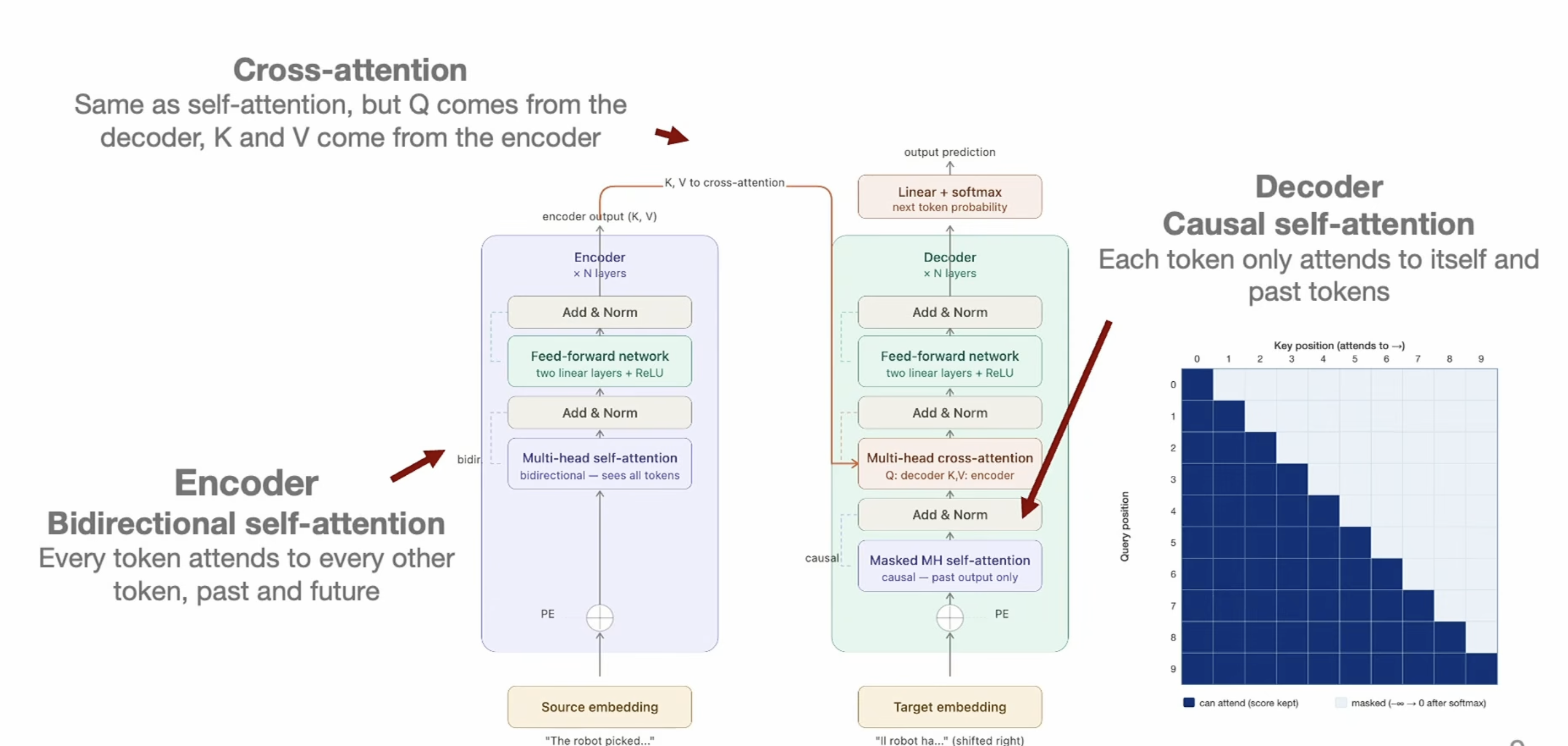
Encoder-decoder Transformer: bidirectional self-attention in the encoder, causal self-attention and cross-attention in the decoder, with the causal mask drawn as a lower-triangular matrix

The slide shows the original encoder-decoder layout and the three flavors of attention that appear in it:

Encoder, bidirectional self-attention. Every token attends to every other token, past and future. This is fine for the input side, which is fully known.
Decoder, causal self-attention. Each token only attends to itself and the tokens before it, enforced by the lower-triangular mask on the right (masked entries are set to $-\infty$ before the softmax, so they get zero weight). This is what makes the decoder autoregressive.
Cross-attention. Same mechanism as self-attention, but the queries come from the decoder while the keys and values come from the encoder output. This is how the decoder reads the input.

Training a Transformer#

Teacher forcing. Maximize the likelihood of the next correct token given the true preceding tokens from the dataset, rather than feeding the model's own (possibly wrong) predictions back in during training. This makes every position in a sequence a training example and lets the whole sequence be trained in parallel.
Cross-entropy loss between the predicted next-token distribution and the actual next token.

Tokenization: Byte-Pair Encoding#

Before any of this, text has to be turned into discrete tokens. Byte-Pair Encoding (BPE) (Sennrich et al., 2016) starts from single characters and repeatedly merges the most frequent adjacent pair into a new token, so common words and subwords end up as single units. A useful property to remember for later: BPE's compression factor scales with the size of the corpus. The more data you learn merges from, the more redundancy it can squeeze out and the fewer tokens a given sequence needs.

Scaling to LLMs#

Getting from "a Transformer" to a large language model is mostly a matter of removing everything that gets in the way of scale:

Decoder-only architectures. Dropping the encoder leaves a single stack of causal self-attention layers, which is simpler to scale and lets one model handle both understanding and generation.
Byte-level BPE. Extending BPE to operate on raw bytes means any string in any language can be tokenized with no out-of-vocabulary tokens.

Two engineering techniques come up repeatedly:

Rotary Position Embedding (RoPE) — a relative positional encoding applied by rotating the query and key vectors, which behaves well as sequence lengths grow.
FlashAttention — an exact attention implementation that tiles the computation to fit in fast on-chip memory, removing the memory bottleneck of materializing the full attention matrix.

The payoff of all this scale is that in-context learning is an emergent property: a large enough model can pick up a new task from a few examples in its prompt, without any weight updates. Nobody designed that in; it appeared with scale.

Extending Transformers to Vision#

The natural next question is how to get images into a model that was built for text. The answer is image tokenization, and the lecture walks through three ways of wiring the visual tokens in:

CLIP — a two-tower contrastive alignment. An image encoder and a text encoder are trained so that matching image-text pairs land close together in a shared embedding space. This gives you a vision encoder that already "speaks" the same space as language.
LLaVA — early fusion. Image tokens are prepended to the text sequence, and the LLM processes everything in a single unified self-attention pass.
Flamingo — late fusion via gated cross-attention. The language model is kept frozen, and visual features are injected through new cross-attention layers whose gates start at zero, so the pretrained LLM is undisturbed at initialization.
Native multimodal models — trained on multiple modalities from the start rather than by bolting vision onto a text model.

The LLaVA case deserves a closer look, because it shows something that matters again when we get to actions. Vision here is input only: the model never has to produce an image token, so image tokens do not need to occupy slots in the vocabulary. LLaVA just needs a way to get them into the Transformer. Compare the two paths:

Text: "cat" → token ID 4937 → embedding-table lookup → 4096-dimensional vector → into the Transformer.
Image: image → ViT → patch features → linear projection → 4096-dimensional vectors → into the Transformer.

Both paths end in the same place, a sequence of vectors the Transformer cannot tell apart. The projection layer is the only new piece.

Putting the progression together: Transformer → LLMs → VLMs → native multimodal models. Each step reuses the previous one and adds a modality.

Extending to Robot Actions: Action Tokenization for VLAs#

If images can be tokenized, can actions? This is the step that turns a vision-language model (VLM) into a vision-language-action model (VLA). Unlike images, actions are outputs, so they genuinely need vocabulary slots the model can emit. The recipe used by RT-2 and OpenVLA is:

Quantile-normalize each action dimension into $[-1, 1]$ . Using quantiles rather than min/max keeps outliers from squashing the useful range.
Discretize $[-1, 1]$ into 256 uniform bins.
An $N$ -dimensional action at timestep $t$ becomes $N$ discrete tokens, one per dimension. All dimensions share the same 256 bin tokens; what distinguishes them is their position in the sequence.
Graft the 256 bin tokens into the LLM's vocabulary. Llama 2 has 32,000 tokens; remove the 256 least frequently used ones and put the 256 action tokens in their place. The model can now output actions, and from its point of view nothing has changed: it is still just predicting the next token.

Action chunking#

This also addresses the third limitation of reactive policies, action smoothness. Instead of predicting one action per query, the model predicts a chunk of $k$ future actions at once.

Paper: Learning Fine-Grained Bimanual Manipulation with Low-Cost Hardware (ACT) (Zhao, Kumar, Levine, Finn, RSS 2023)

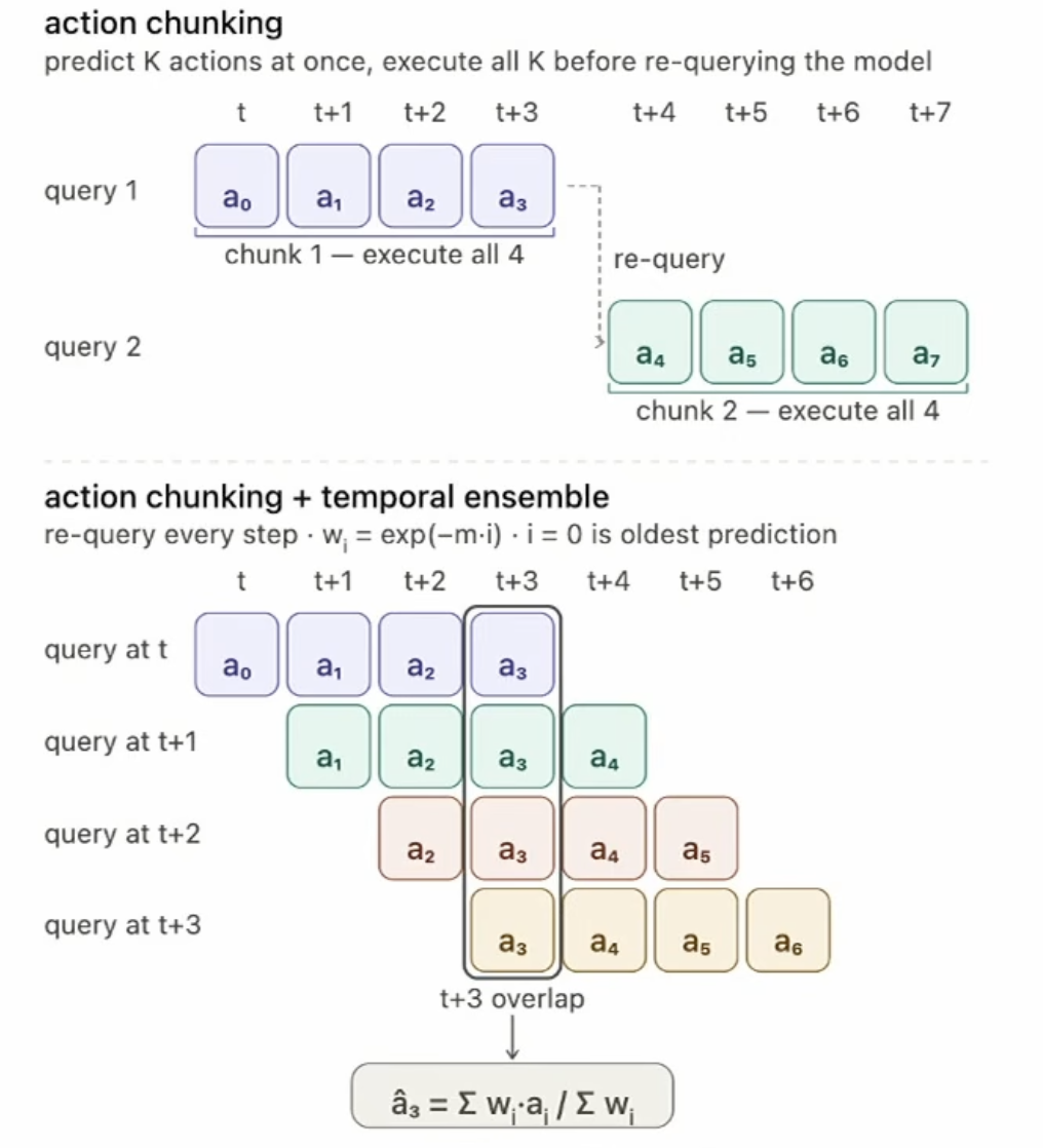
The slide shows two variants:

Plain action chunking. Predict $K$ actions, execute all $K$ , then re-query the model. Fewer queries, and each chunk is internally consistent, so the motion is smoother.
Action chunking with temporal ensembling. Re-query at every step, so several chunks overlap at each timestep. The executed action is a weighted average of all predictions for that timestep, $\hat{a}_t = \sum_i w_i a_i / \sum_i w_i$ with $w_i = \exp(-m \cdot i)$ , where $i = 0$ is the oldest prediction. This smooths out the jumps at chunk boundaries.

ACT (Action Chunking with Transformers) is the model that made this work for dexterous, fine-grained bimanual manipulation on low-cost hardware.

The problem with high control frequencies#

Naive binning tokenization runs into trouble as the control frequency goes up, for two related reasons: the information per token decreases, and the correlation between neighboring tokens increases.

Take a single task — "pick up the spoon on the table" — and assume it takes 4 seconds with a 7-dimensional action:

Control frequency	Timesteps	Tokens
10 Hz	40	280
50 Hz	200	1400

The key point is that both rows describe the same task and contain exactly the same amount of information. Reach, align, close the gripper, lift: the decisions that have to be made are those few, and they do not multiply because you sample five times faster. So the information carried by each token is simply diluted five-fold.

What happens next is the dangerous part. Because the Transformer is autoregressive, the model discovers that it can just copy the previous token's value. That is not hard to learn: it only has to look back a fixed number of positions. Cross-entropy loss is determined entirely by the conditional distribution, and in high-frequency data "the next step equals the previous step" is extremely likely, so guessing "same as before" already drives the loss very low.

Gradient descent is greedy. It finds the cheap path first, and once the copy circuit has formed, the loss is already low and the remaining gradient is too weak to push the model down the expensive path of actually modeling the task. The model gets stuck in a local solution, and that solution looks perfectly good on the loss curve.

Task success score of naive binning tokenization versus data control frequency: it peaks around 5 Hz and collapses toward zero at 10 Hz and 20 Hz

Paper: FAST: Efficient Action Tokenization for Vision-Language-Action Models (Pertsch, Stachowicz, Ichter, Driess, Nair, Vuong, Mees, Finn, Levine, 2025)

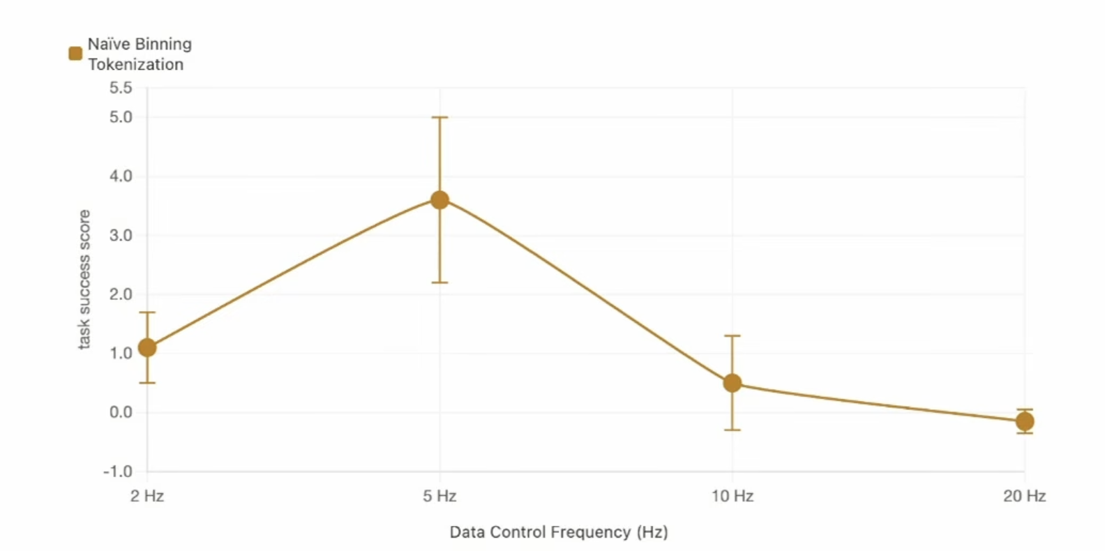
The plot makes it concrete. With naive binning, task success is best around 5 Hz and falls to essentially zero at 10 Hz and 20 Hz, exactly the frequencies you want for dexterous control.

The fix: compress before you tokenize#

FAST's logic follows directly from the diagnosis. If the problem is redundancy, squeeze the redundancy out before tokenizing:

DCT. Apply a discrete cosine transform to the whole action chunk, moving it into the frequency domain. For a smooth trajectory almost all of the energy sits in the low-frequency coefficients; the high-frequency coefficients are close to zero and can simply be dropped.
BPE. Encode the remaining quantized coefficients with byte-pair encoding, which folds the frequently co-occurring patterns into single tokens.

The result is an order of magnitude fewer tokens, and, more importantly, every token now carries real information. Neighboring DCT coefficients are not correlated with each other, so "copy the previous coefficient" is a useless strategy. The shortcut is closed off architecturally, and the model has no choice but to learn the actual structure of the task.

Closing Thoughts#

Why does this lecture exist in a robot learning course? Because robotics is a sequence modeling problem, and the most common and mainstream way to do sequence modeling today is with a Transformer. Reading the notes back, the chain is:

Partial observability forces the policy to condition on history, which makes it an autoregressive model.
Transformers are the autoregressive model that scales, and the LLM playbook (decoder-only, byte-level BPE, RoPE, FlashAttention) is how they scale.
Vision slots in as extra input tokens through a projection layer; no vocabulary changes needed.
Actions are outputs, so they need real vocabulary slots, and how you tokenize them decides whether the model learns the task or learns to copy. Chunking buys smoothness; FAST's compression buys tokens that are actually worth predicting.