Learning One Representation to Optimize All Rewards

This post shares the paper Learning One Representation to Optimize All Rewards. As the title suggests, it addresses a long-standing problem in reinforcement learning: needing a separate policy for every single reward. The paper proposes a method called the FB-representation, which trains a model without requiring a reward function up front, and can still reach a near-optimal solution once a reward function is provided afterward.

Background knowledge#

Value-based RL

Q(s,a)=\sum_{s'}P(s'|s,a)\left[R(s,a,s')+\gamma\max_{a'}Q(s',a')\right]

How to get the policy from Q-value

\pi(s)=\arg\max_a Q(s,a)

Introduction#

We consider one kind of unsupervised reinforcement learning problem: Given a Markov decision process (MDP) but no reward information, is it possible to learn and store a compact object that, for any reward function specified later, provides the optimal policy for that reward, with a minimal amount of additional computation? In a sense, such an object would encode in a compact form the solutions of all possible planning problems in the environment. This is a step towards building agents that are fully controllable after first exploring their environment in an unsupervised way.

Goal-oriented RL methods compute policies for a series of rewards specified in advance (such as reaching a set of target states), but cannot adapt in real time to new rewards, such as weighted combinations of target states or dense rewards.

Learning a model of the world is another possibility, but it still requires explicit planning for each new reward; moreover, synthesizing accurate trajectories of states over long time ranges has proven difficult in practice.

Instead, we exhibit an object that is both simpler to learn than a model of the world, and contains the information to recover near-optimal policies for any reward provided a posteriori, without a planning phase.

One line of prior work learns optimal policies for all rewards that are linear combinations of a finite number of feature functions provided in advance by the user. This limits applications: e.g., goal-oriented tasks would require one feature per goal state, thus using infinitely many features in continuous spaces.

🧠 My take: the framing here is what makes the paper interesting to me — most RL work treats "the reward" as a given, fixed thing you train against. Flipping that around (learn something reward-agnostic first, plug in the reward later) is the same move that made pretrained embeddings useful in NLP and vision. If it works, it turns "train a new policy" into "do a bit of linear algebra."

Prior approaches

Universal Successor Features Approximators, USFA

Mechanism: linear combination of predefined features

The core idea assumes that any possible reward function $r(s, a)$ can be expressed as a linear combination of a finite, predefined set of feature functions $\phi(s, a)$ .

How it works: The user must supply a set of features $\phi$ before training. The system then learns a "Successor Features" function $\psi$ , representing the discounted future accumulation of those features.
Advantage: If a new task's reward really is a linear combination of these features, the agent can switch policies quickly just by swapping the weight vector $w$ .

Limitations: feature explosion and the continuous-space problem

USFA has real practical limitations:

Lack of flexibility: It can only handle rewards that are linear in the predefined features $\phi$ , not more complex or nonlinear reward functions.
Trouble with goal-oriented tasks: For goal-oriented tasks where the reward is "reach a specific state $s_g$ ," a corresponding feature (e.g., an indicator function $\delta_{s,s_g}$ ) must be defined for every possible goal state.
Challenge in continuous spaces: In continuous spaces there are infinitely many states. Being able to reach "any" location would in theory require infinitely many feature functions, which is computationally impossible.

Mathematical formulation

Definition of the reward function
$r(s, a) = \phi(s, a)^\top w$

The reward is assumed to be a weighted linear combination of the feature $\phi$ : $\phi$ is the user-provided feature vector, and $w$ is the weight corresponding to a specific task.

The central concept of this paper is the Successor Measure described below.

Successor Measure#

Successor Features, $\psi$
$\psi(s_0) = \sum_{t \geq 0} \gamma^t\, \mathbb{E}[\phi(s_t) \mid s_0]$

The system learns a function $\psi$ that predicts the distribution of future features (a simplified version that ignores actions): this represents the discounted sum of feature $\phi$ observed in the future, starting from state $s_0$ under a given policy.

Computing the Q-function
$Q(s, a, w) = \psi(s, a)^\top w$

At test time, given the weight $w$ , the Q-value can be obtained directly via a dot product:

Weight estimation
$w = \big(\mathrm{Cov}_{\rho_{\text{test}}}(\phi)\big)^{-1} \; \mathbb{E}_{(s, a) \sim \rho_{\text{test}}} \big[\,r(s, a)\, \phi(s, a)\,\big]$

At test time, $w$ is typically estimated from observed rewards via linear regression:

This expression can be understood in two parts:

$\mathbb{E}_{(s,a)\sim \rho_{\text{test}}}[\,r(s,a)\,\phi(s,a)\,]$ (numerator): This computes the correlation between the reward $r$ and the feature $\phi$ . If a feature is especially prominent wherever the reward is high, this expectation will be large, meaning that feature contributes strongly to the reward.
$\big(\mathrm{Cov}_{\rho_{\text{test}}}(\phi)\big)^{-1}$ (denominator): This is the inverse of the features' covariance matrix, and it acts as a normalizer. Since different features may overlap or have different scales, this matrix removes correlation between features, ensuring the computed $w$ is the most precise weight without double-counting.

🧠 My take: this weight-estimation step is the part I find most elegant. Once you already have $\phi$ , recovering $w$ is just linear regression — no gradient descent, no fine-tuning, nothing reward-specific to train. That's the whole promise of the paper in miniature: push all the hard learning into a reward-free phase, and make the reward-specific phase closed-form.

This paper reuses a similar policy parameterization, but introduces a novel representation with better properties, based on state occupancy prediction instead of expected featurizations, building on prior theoretical advances in successor-state learning. This gives us the following.

Encoding All Optimal Policies via the Forward-Backward Representation#

Successor Measure

As the measure over $S \times A$ representing the expected discounted time spent in each set $X \subset S \times A$

In the discrete-state case:

Q^\pi_r(s,a) = \sum_{s',a'} M^\pi(s,a,s',a')\, r(s',a')

Because the $Q$ -function relates to reward $r$ as $Q = Mr$ (i.e., cumulative value equals the product of future occupancy and reward), the value of any policy $\pi$ defined by a parameter $z$ , for any reward $r$ , can be written as (writing $F_z(s,a) := F(s,a,z)$ for brevity):

Q^{\pi_z}_r = (F_z^\top B)\, r = F_z^\top (Br)

where

z_r := B r

Since

\pi_{z_r}(s) = \arg\max_a \big(F_{z_r}(s,a)^\top z_r\big)

by the Bellman Optimality Equation.

In continuous spaces, we instead work with its density function $m^\pi$ . The core goal of the FB representation is to train two neural networks, $F$ and $B$ , such that their dot product approximates this density:

F(s, a, z)^\top B(s', a') \approx m^{\pi_z}(s, a, s', a')

Relation to the Q-value: Once this measure is available, computing the Q-value for any reward function $r$ becomes a simple integral (or dot product):
$Q^\pi_r(s_0,a_0) = \int r(s,a)\, M^\pi(s_0,a_0,\mathrm{d}s,\mathrm{d}a) = \int r(s,a)\, m^\pi(s_0,a_0,s,a)\, \rho(\mathrm{d}s,\mathrm{d}a)$ $\approx F(s_0,a_0,z)^\top \underbrace{\int r(s,a)\, B(s,a)\, \rho(\mathrm{d}s,\mathrm{d}a)}_{z_R} = F^\top z_R$

Continuous-case formula:

M^\pi(s_0, a_0, \mathrm{d}s, \mathrm{d}a) = m^\pi(s_0, a_0, s, a)\, \rho(\mathrm{d}s, \mathrm{d}a)

z_R := \int_{s,a} r(s,a)\, B(s,a)\, \rho(\mathrm{d}s,\mathrm{d}a)

Prior work proposes an update rule that learns this density without needing a reward signal:

\delta\theta := \underbrace{\partial_\theta\, m^\pi_\theta(s_0, a_0, s_0, a_0)}_{\text{first term: self-occupancy}} \;+\; \underbrace{\partial_\theta\, m^\pi_\theta(s_0, a_0, s', a') \times \big[\gamma\, m^\pi_\theta(s_1, a_1, s', a') - m^\pi_\theta(s_0, a_0, s', a')\big]}_{\text{second term: TD propagation}}

Breaking down what this means:

First term (self-occupancy): This corresponds to time $t=0$ and forces the model to acknowledge: if I'm currently at $(s_0, a_0)$ , then the density of "arriving" at $(s_0, a_0)$ must be high. This resolves the zero-probability problem in continuous spaces.
Second term (TD error): This is a standard temporal-difference term. It states: "the probability of reaching a distant target $s'$ from $s_0$ should equal the (discounted) probability of reaching $s'$ from the next step $s_1$ ."
Key advantage: Instead of a sparse reward that gives 1 only upon reaching the goal and 0 otherwise, it uses every environment transition $(s_0, s_1)$ to update the map, since every step arrives "somewhere."

🧠 My take: this self-occupancy trick is the quiet hero of the method. In continuous space, "the probability of being exactly at one point" is technically zero, which would normally kill the reward-free training signal entirely. Anchoring the model at $t=0$ sidesteps that without needing any handcrafted sparse reward — it's a small fix, but it's the reason the density can be learned from raw transitions alone.

Evolving into FB: Introducing the Policy Parameter $z$ #

The original successor-state algorithm above can only learn the map for one fixed policy $\pi$ . FB's innovation is extending this to infinitely many policies.

Model substitution: FB replaces that single model $m^\pi(s, a, s', a')$ with the dot product of two neural networks:

m^{\pi_z}(s, a, s', a') \approx F(s, a, z)^\top B(s', a')

Role of the parameter $z$ : Here, $z$ is a randomly sampled vector representing a kind of "virtual task goal."
Training logic: During training, the algorithm randomly samples a $z$ , then defines the corresponding policy $\pi_z(s) = \arg\max_a F(s, a, z)^\top z$ .

🧠 My take: this is basically a universal value function ( $z$ standing in for "the goal") wearing a different hat. What's neat is that $z$ never has to be an actual goal state — it's just some vector, sampled at random, and the network is forced to make its own notion of "task" out of that. That's what lets FB generalize past goal-reaching to arbitrary reward functions later.

FB's Final Loss Function#

Combining the concepts above yields FB's unsupervised loss function:

L(\theta, \omega) = \mathrm{MSE}\Big(F(s_i, a_i, z_i)^\top B(s'_j, a'_j),\ \ \gamma\, F(s_{i+1}, a_{i+1}, z_i)^\top B(s'_j, a'_j)\Big) \;-\; \text{(self-correction term)}

What is this equation doing?

Left side ( $F^\top B$ ): The model predicts the reachability of the target state from the current state.
Right side ( $\gamma F^\top B$ ): Uses the prediction from the next state as the TD target.
Subtracted term (self-correction): This is the self-occupancy term from earlier, ensuring the model doesn't learn all reachability as 0 — it forces the model to output a high value when "start = end."

🧠 My take: it's worth noticing this loss is entirely self-supervised — no reward $r$ appears anywhere in it. That's the whole trick made concrete: $F$ and $B$ are trained purely from state transitions and a randomly sampled $z$ , and the reward only enters much later, at inference time, through the closed-form $z_R = \mathbb{E}[rB]$ . That separation is what makes the "one representation, any reward" claim actually work rather than just sound good.

Summary: How Is It Used?#

FB cleverly leverages the successor-state approach's ability to learn "long-term relationships between states," with two major improvements:

Structuring: Decomposing the density into Forward and Backward components. This turns $B$ into an automatically learned "feature extractor," while $F$ becomes the "predictor."
Generalization: By continuously varying $z$ during training, $F$ and $B$ are forced to learn a summary of all possible paths in the environment.

Final result: Once trained, this mathematical structure becomes a "pre-computed answer book." Given a new task $r$ , you only need to compute

z_R = \mathbb{E}_{(s,a)\sim\rho}\big[\,r(s,a)\, B(s,a)\,\big]

and then

F^\top z_R

directly becomes the Q-value function for that task, with no need for any further path search or planning.

🧠 My take: this is effectively "zero-shot RL" — you never touch the reward during training, yet you get a usable policy for it in one linear-algebra step at test time. The obvious question I'd want answered next is how near-optimal $F^\top z_R$ really is compared to a policy trained end-to-end on that specific reward, and how that gap behaves as the environment gets more complex than a four-room maze.

Experimental Results#

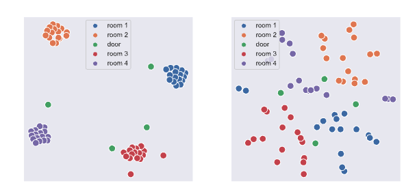
Picture a square room with cross-shaped walls dividing it into four smaller rooms (Room 1 through Room 4), connected only by a small door in the center. This is the maze the AI practices navigating.

What do the dots in this figure represent?

Each colorful dot in the figure represents a specific coordinate (location) in the maze.

Physical space: In the actual maze, these points are arranged in a regular grid.
The AI's logical space: The figure above shows what these coordinates look like after the AI converts them into "feature vectors" and projects them onto a plane.
How to read it: If two points in the figure are close together, it means the AI considers those two locations "logically connected" (easy to reach from one another); if they're far apart, the AI considers those locations blocked off from each other (e.g., by a wall in between).

A closer look: left plot vs. right plot

Left plot: Forward representation (F embedding) — the "map of future paths"

This reflects the AI's understanding of "starting from here, where can I go in the future."

Four large clusters: You'll see the points naturally group into four clusters. This shows the AI has discovered that as long as you're in the same room, your "future possibilities" are very similar.
Gaps (walls): The large empty spaces between clusters are the walls the AI has "sensed." Even though it never saw the actual map, it discovered that points in the top-left can never directly move to the bottom-right, so it logically places these two groups of points very far apart.
Green points (doorways): Notice a few green dots between the clusters. Those are doorways — the AI has discovered these points are the only "bridges" letting it jump from one cluster (room) to another.

Right plot: Backward representation (B embedding) — the "ID card" of a location

This reflects the AI's understanding of "who am I, where am I" — it's a label used to distinguish different locations.

Why does it look more scattered? This is because a mathematical constraint in the algorithm (orthogonalization) forces the AI to give each location a unique identifier, preventing points from clustering together, so that positioning stays precise once a task (reward) is given.
Still structured: Even though the points are more scattered, if you look closely at the colors, points from the same room still roughly stay within the same region — showing the map's structure is still preserved.

🧠 My take: the F/B split really is the paper's core idea made visible — F clusters by "where can I still go" (a planning-shaped view), B clusters by "which exact point am I" (an identity-shaped view). Seeing the four rooms fall out automatically, with zero access to the maze layout, is a nice sanity check that the density-matching objective is actually learning the environment's connectivity and not just memorizing coordinates.

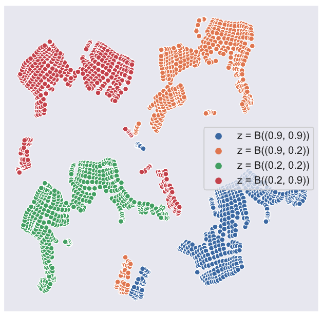
This figure provides further visualization of the forward representation (F embedding) under different goal orientations, in the continuous maze environment.

Different colors represent different "task vectors z"

Four colors are used in the figure, each representing a different task vector $z$ (computed as $z = B(\text{goal coordinate})$ ):

Blue: goal in the top-right corner (0.9, 0.9).
Orange: goal in the bottom-right corner (0.9, 0.2).
Green: goal in the bottom-left corner (0.2, 0.2).
Red: goal in the top-left corner (0.2, 0.9).

The F Embedding Changes Dynamically with the "Goal"#

This is the most central property of the FB representation: the forward representation $F$ is a function of $z$ (i.e., $F(s, a, z)$ ).

You can see that as the goal ( $z$ ) changes, the AI's "internal representation" of the same physical location shifts to a different region of the space.

The Core Meaning of These Plots#

Policy parameterization: This figure visually demonstrates that the AI has indeed learned a family of policies parameterized by $z$ . Give it a different destination, and its internal "predictive summary" of the environment immediately adjusts to match the logic of reaching that goal.
Logical separation: The four colors of points are spread far apart, showing that the AI has entirely different understandings and processing paths for "going to the top-right" versus "going to the bottom-left" in the embedding space.
Preserved spatial structure: Even though the points shift depending on the goal, points within each color still maintain some degree of spatial proximity (points that were originally close remain relatively close in the projection), showing that it still respects the connectivity of the physical environment.
Left-hand side $M^\pi\big(s_0,a_0,\{(s',a')\}\big)$ : represents how long, starting from $(s_0,a_0)$ under policy $\pi$ , the agent is expected to spend at $(s',a')$ in the future (expected discounted occupancy time).
Right-hand side, first term $\mathbf{1}[s_0=s',\, a_0=a']$ : this is the "current" state. If you're currently at the target point $(s',a')$ , the value is 1; otherwise it's 0.
Right-hand side, second term $\gamma\, \mathbb{E}[\cdots]$ : this is the "future" expected occupancy — the total time to reach the target point $(s',a')$ starting from the next state $s_1$ , discounted by factor $\gamma$ .

🧠 My take: this plot is the clearest evidence in the paper that $z$ is doing real work rather than just being a free parameter. If the embeddings didn't reorganize per goal, you'd suspect $F$ had collapsed to ignoring $z$ entirely and just memorizing a single default policy. The fact that "same location, different goal" lands in visibly different regions is what makes me believe the multi-policy claim, not just the loss curve.

In short: this describes how "the probability of being at $(s',a')$ if that's where you want to go" equals the sum of "being there right now" plus "arriving there after the next step."